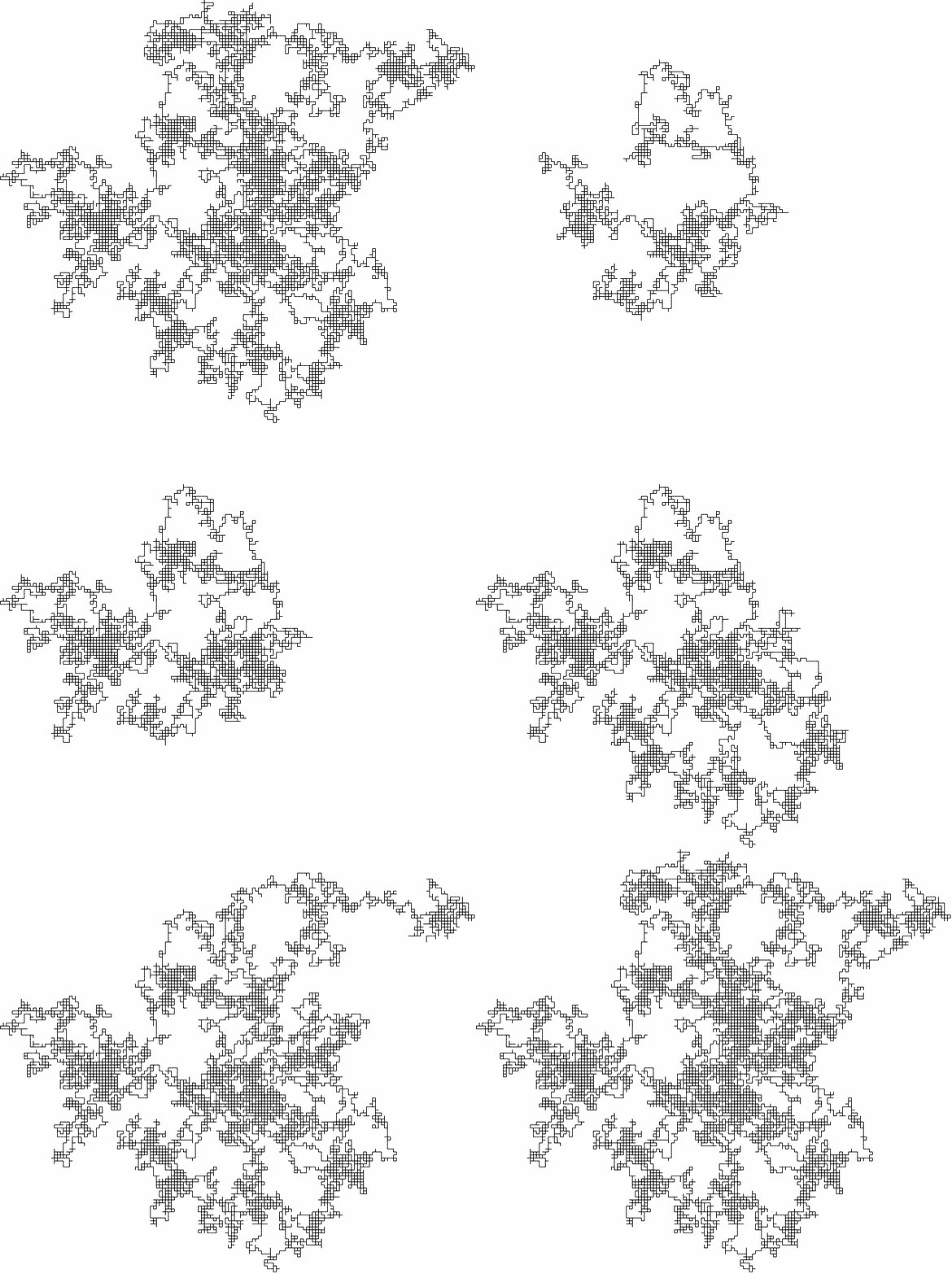
Casino can teach you a lot about Stochastic Processes and Uncertainty than a textbook would do, the only trade off is that there are comparatively higher chances that the former would bring you to streets than the latter.Random walk is a famous stochastic model used for many applications.
It can be best explained using a popular challenge called Gambler Ruins Problem. Let’s say that we have two players A and B who share Rs. T. At each and every round, the winning player is owed a rupee from the loosing one. Now, let’s assume that the player A wins a particular round (He/She gets a rupee from player B) with some probability p in the range (0,1). This directly means that winning probability for player B is 1 - p. This game ends if either of them looses all of their money on this ( We say that the loosing player is ruined ).
In context with Stochastic Models, once the problem definition becomes clear, the first step is to define the process itself. Let Xn be the amount that is owned by the Player A at time step n. Then, T - Xn is the amount owned by Player B. Xn will belong to this set {0,1,2,…,T}. Then,
Once the definition of stochastic process is done, the next step is to define the Transition Probabilities. We will have to define success and failure in this context before that. As usual, let’s assume that player A wins if he/she gets a head as an outcome of an unbiased coin toss (the outcomes of this random experiment are equally likely), and otherwise for player B. As a result, the transition probability matrix would look something like this (from the perspective of player A )
| T | 0 | 1 | 2 | 3 | 4 | … | t-1 | t |
|---|---|---|---|---|---|---|---|---|
| 0 | 0 | 1 | 0 | 0 | 0 | … | 0 | 0 |
| 1 | 0.5 | 0 | 0.5 | 0 | 0 | … | 0 | 0 |
| 2 | 0 | 0.5 | 0 | 0.5 | 0 | … | 0 | 0 |
| 3 | 0 | 0 | 0.5 | 0 | 0.5 | … | 0 | 0 |
| 4 | ||||||||
| … | ||||||||
| t-1 | 0.5 | |||||||
| t | 1 | 0 |
Now you might ask, how is this even relate to random walk ?
The following figure illustrates a Random Walk
